Large DNNs And Bad Local Minima

This is a follow-up post to Large DNNs Look Good, But They May Be Fooling Us.

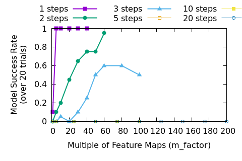
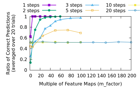
In that post we looked at training a DNN to solve Conway’s Game of Life over different numbers of steps.

Let’s look at the success results from the previous post. To refresh our memory, “success” means that the DNN correctly predicted the dead or alive status for each cell after the given number of steps, tested over 1000 5x5 initial states.

Figure 1. Likelihood of complete model success over 1000 tests after training to predict more steps steps in the Game of Life. Success drops with increased steps.

Figure 2. The success rates for individual tiles over all of the 20 trained models. A success rate of 0.5 is what we expect if the network is just “guessing”.

Let’s spend a moment discussing how a deep neural network (DNN) “learns”.

What is “learning?”

When we talk about the learning process in a DNN, we are describing the way that weights and biases are adjusted by stochastic gradient descent (SGD). Each variable that has some effect on the end result shares some part of any error: this is called the “gradient.” There are cases when the gradient is 0, such as when a variable goes through a function that zeros the output, such as ReLU, or when operations withing a network structure drop the gradients towards zero, called the vanishing gradient problem.

We know that our DNNs are larger that strictly required to solve the problem where they are applied. It is common to apply something like L1 or L2 loss to force some parameters to 0 and then prune them after training so that the end result is a smaller network. A regularizer like dropout can accomplish the same thing (I should make a post about this, but imagine a system with 2 inputs, one of which is noisily correlated with the desired output and the other which can be used to derive the output exactly–dropout can be used to force the weight of the noisy input to 0).

To get a “good” gradient, there must exist some parameters that have an output that is close to the correct one such that a “path” over the loss surface (the loss values over different values of the DNN’s parameters) exists that is mostly downhill from the starting point to the correct answer. Thus the parameters follow the gradient and “descend” into the global minima of the loss.

But what if all of the parameters get into a position where going towards the correct answer would make them go up hill? This is a local minima, and the networks that were being trained to solve the game of life were certainly getting stuck in them.

For an example of a local minima, imagine that the DNN is detecting every single possible starting configuration of 0’s and 1’s and mapping them, one by one, onto the correct outputs. There are $2^9$ possible states in a 3x3 filter’s receptive field, so that would take 2048 filters to brute force.

Let’s say that things don’t go so badly and the weights of the corner positions, which are uncorrelated with the desired output, go to 0 quickly. Now there are $2^5$ filters to find, which is only 32. Let’s say that the DNN quickly learns 30 of them–but there are only 30 filters in that layer. The DNN will be stuck, because if it changes any of the existing filters it will get worse and the loss will go up. Each of the existing filters leads to a “correct” output $30/32$ times, so the training loss won’t pull them out of their current states. The DNN is now stuck in a local minima.

That isn’t even a worst case–at least some of the outputs are correct. Imagine a case where the gradient sometimes pulls values one way and sometimes pull them in another way, but never pulls very strongly. Those parameters will get “stuck” because the loss surface is too flat. Now, if some of the desired outputs are “solved” by other parameters the loss for those cases will go down, freeing those parameters to move to solve the inputs that still lead to high loss, but one the DNN gets stuck that can no longer happen.

This is perhaps difficult to visualize, so let’s try to take a look at some real examples.

Figure 3. The change in loss over a “walk” from a minimal correct solution to various local minima from 10 different training runs. The model is predicting a single step in the game and has no extra capacity. Observe that even thought the starting position has a lower loss than the result from training, the path from one to the other has one or more areas of positive slope so gradient descent will not avoid the local minima.

Figure 4. The loss walk from a minimal solution to another 10 trained models, this time with the number of filters per layer multipled by 5 (m_factor = 5). Observe that the loss surface is smoother and the the local minima are acceptable solutions.

Figure 5. The loss walk for 2 steps with m_factor = 1. The loss surface is not smooth and SGD is easily trapped in local minima far from a good solution.

Figure 6. The loss walk for 2 steps with m_factor = 5. As in Figure 3 the loss surface is smoother with the additional layers, but it there are still minima where the training progress can become stuck. The complexity of the loss surface increases with the number of steps.

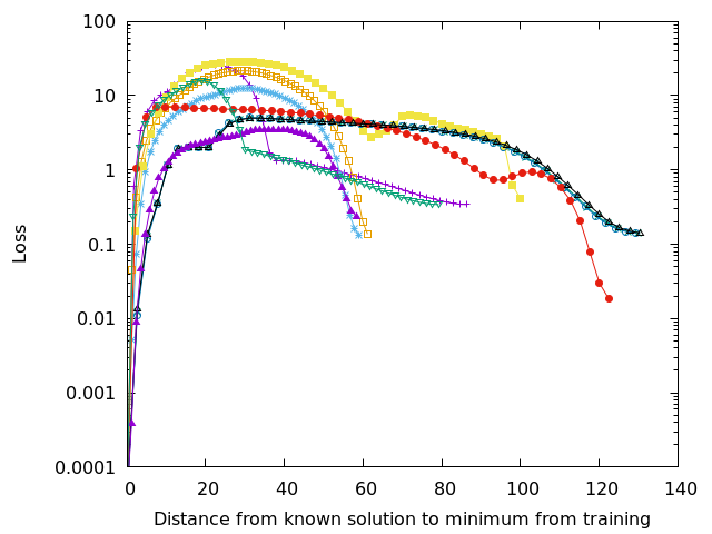
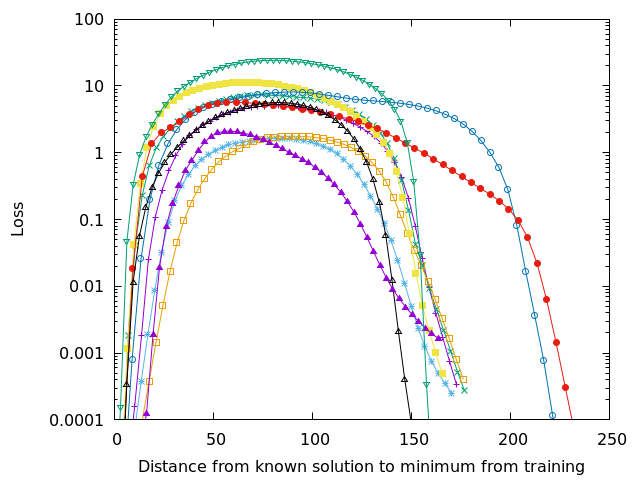
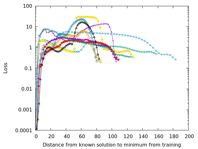
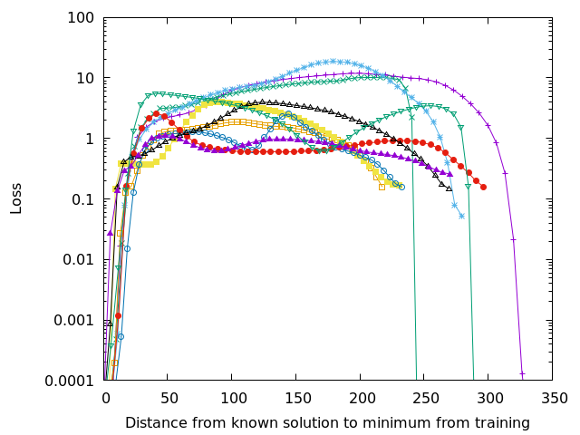
Each of the lines in Figures 3-6 show a walk from a known high quality solution (as described in the previous post) to the solution found during training. Since the loss surface has as many dimensions as there are parameters in the network, it isn’t easy to visualize–but if you’re a higher dimensional being you can think about it as an n-dimensional mountain range. Each of the lines on those figures represents a straight line walk from one point to another along the loss surface. The peaks–those areas with extremely high loss– separate the loss surface into discrete zones.

Some textbooks may pretend that a complicated route through several valleys will connect any starting position to similar local minima, but that isn’t true in this case and is very likely untrue in practice. The initial starting position, the random initialization of the DNN’s weights and biases, will determine where training will converge. On each figure you can see that several of the lines end up at nearly the same location, so training can converge to the same (or nearly the same) solution. The important question is whether or not that solution is any good.

Adding more parameters to the DNN smooths out the loss surface and may join some of the loss valleys together. Smoothness helps, but it is still possible to get an unlucky initialization of a network, which is probably why in practice we always train several networks for a task rather than a single one. In academic papers we then report statistics and in industry we select the best model for deployment. This is yet another overhead cost of the brute force approach of current training techniques.

Unknown Magic

A general solution to this is unclear, at least to me. Replacing stochastic gradient descent with some unknown magic would be nice, but the fact is that no human that I know of is anything more than a metaphorical wizard. It is possible that changing the problem space would improve the loss surface, so one possibility would be to change the way that we use DNNs for predictions.

For example, instead of making a DNN that distinguishes between multiple different classes we could train a DNN that detects the various qualities of an object: is it metal, does it have wings, is it currently flying, etc. Individual qualities can be used to distinguish between object classes while being more straightforward to label and train. DNNs could also be trained to output trees that capture the relationship between classes, which would better capture relationships between them and could allow for the DNN to express confidence up to a point–this also requires more work when creating labels though.

Another thing to think about is that we allow DNNs to give us meaningless answers because of the way that we train them. Maybe we should stop? When we put a softmax at the output of our classifiers, we force those outputs into a range that looks correct, regardless of what nonsense is coming out of the last layer of the network, effectively hiding the state of the network outputs.

For example, a softmax converts its inputs so that they all sum to 1, as a probability should, even though the outputs aren’t really probabilities. These DNNs will rapidly learn any local features that are highly correlated with particular object classes since those gradients are likely present through the loss surface. This can lead to trained DNN’s with outputs that depend upon local textures rather than a discrete set of features that uniquely define an object of a particular class, which in turn makes those DNNs vulnerable to adversarial attacks or to unexpected failures.

Most troubling, many trained DNNs do not allow for the network to output low confidence for all object classes. If the responses of the different convolution filters in the network are weak then the output of the softmax becomes quite noisy. This happens at training time as well as during inference, meaning that we are training on noise as if it were meaningful.

DNN practitioners are well aware that the outputs of a softmax classifier can’t be treated as real probabilities, so a change in the outputs of DNN classifiers wouldn’t actually cause much disruption to their users.

I will do my best to keep the complicated nature of loss surface in mind as I train neural networks, and I think it best that any other user of DNNs does the same. Just because the loss goes down during training doesn’t mean that the place where we end up is any good. Even when results seem to be “good enough,” that is no excuse to avoid looking for a better result.