Paper Review: Limits On Learning Machine Accuracy Imposed by Data Quality

This paper, published in 1994 and written by Corinna Cortex, Larry Jackel, and Wan-Ping Chiang, is both a good read and is still relevant for today’s machine learning researchers. As was the case with many papers of the time, it was written with a clear, direct style to inform colleagues of something interesting and important. It lacks the overly complicated equivocation of modern papers, which are often written by torturing phrases until they lie still on the page to create an illusion of careful planning and rational design. The paper only cites a mere 8 references, which makes it quite easy to check the state of research at the time. It’s a breath of fresh air compared to modern papers that have a page or more of references lurking at the end.

The paper describes why learned models exhibit an upper bound on their performance as a function of their data quality. The data that they analyzed was from failures in a telecommunication system, which was relevant to the AT&T network at the time. It may not feel relevant to a machine learning researcher in the 2020s, but the paper’s methodology is insightful. I will endeavor to both explain the paper and to show how it is relevant in the modern world of enormous datasets and billion parameter models.

First, let us begin with the supposition that before you begin swinging your machine learning cudgel around to smash every problem within reach you, as a rational being capable of complex behavior, first take a few moments to estimate the upper bound of what is achievable with your statistical model. For example, if you are attempting to predict the state of a fair coin after flipping it you would be wise to only promise 50% accuracy from your model since a fair coin is random. Most problems we try to solve are less random than that, but it is rare that we can expect 100% success with any system.

First I’ll discuss the contents of the paper. Afterwards, I will draw two examples from modern machine learning, specifically ImageNet and autonomous vehicles, to illustrate how those ideas can be applied.

Here is the key point of the paper, as stated at the end of section 1:

We conjecture that the quality of the data imposes a limiting error rate on any learning machine of ~25%, so that even with an unlimited amount of data, and an arbitrarily complex learning machine, the performance for this task will not exceed ~75% correct. This conjecture is supported by experiments.

The relatively high noise-level of the data, which carries over to a poor performance of the trained classifier, is typical for many applications: the data collection was not designed for the task at hand and proved inadequate for constructing high performance classifiers.

It’s a fact of life that all data has noise in it, although what is meant by the term “noise” can vary from one dataset to another. We would like to believe that clever tricks and bigger models make this problem go away, but this is, unfortunately, not the case. While we do have better techniques to deal with mismatches between training and testing data than when this paper was written, we do not have a method that can completely ignore the presence of noise in our datasets.

Before going farther though, I’m going to reproduce some of the figures from the paper so that we can all share a common vocabulary for this discussion.

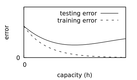
First, let’s talk about the match between training and testing data. Figure 1 shows an idealized error as we increase our model capacity if the training set data and test set data do not match. This is commonly called “overfitting.” Overfitting cannot happen when the training and testing data match. Now, getting training and testing to match completely is impossible, but for practical purposes if the number of training examples is great enough then the model will not have enough parameters to simple learn each of those examples individually and it must generalize.

Of course, in modern machine learning we employ gigantic models with gleeful abandon, and with seemingly no ill-effects. We can get away with this if we use strong regularizers. These techniques enforce sparsity in the model, which resists fitting parameters that only apply to small number of examples from the training set.

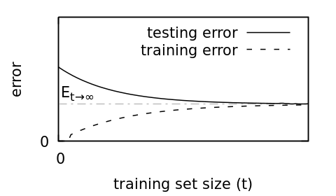
One thing that has not changed over time is machine learning’s hunger for data. More data means that we can increase our model size and increases the likelihood that our training data covers all of the examples in our test set. This leads to a convergence of error between training and testing data, as shown in Figure 2. Ideally we would increase our training set until all of our errors reach zero. However…

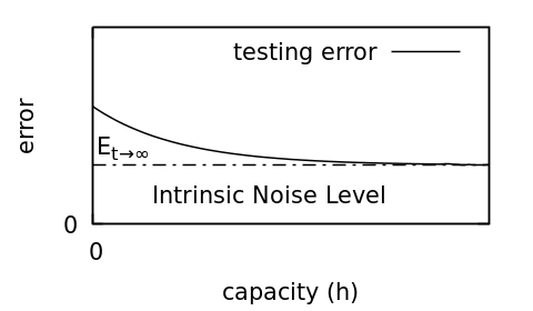
As illustrated in Figure 3, this is not realistic because our data is always flawed. That doesn’t mean that we can’t estimate the error stemming from the quality of our data. Doing so is helpful. If the errors that will come from the data are below the acceptable errors of the system then we can ignore them. If not, then we need to find a way to improve our data quality.

Knowing the expected error threshold also helps us to see when there are no more gains to be made with a dataset. This can save you from wasting a limitless amount of time trying to perform an impossible task.

Let’s jump into those modern examples, starting with ImageNet.

The ImageNet challenge, formally the ImageNet Large Scale Visual Recognition Challenge (ILSVRC), has image scraped from around the Internet that belong to one of 1,000 different classes. There are more than 1.2 million training images, 50,000 validation images, and 100,000 test images. Labelling was crowdsourced with Mechanical Turk, so the labels are questionable. If we check paperwidthcode, we will learn that “Top-1 Accuracy”, meaning the accuracy with the highest probability class label, cleared 90% in early 2020 when EfficientNet-L2 achieved 90.2% accuracy. Since then, the highest classification accuracy has ascended too… 91.1%.

So, why not 100%? Let’s do as the authors of “Limits On Learning Machine Accuracy Imposed by Data Quality” and check for ourselves.

Consider the related classes: “toilet_tisuee” and “toilet_seat” (yes, these are really two of the 1,000 classes in ILSVRC). Clearly there can be some overlap here. How much? I checked the 1,300 examples of toilet seats and found that 195 of them contained toilet paper (in some form–my count is likely imperfect, but I will not be looking through 1,300 pictures of toilets for a second time). This means that 15% of the toilet seat images could be legitimately labelled toilet tissue instead.

Now, I didn’t check for any of the other 998 classes inside of the toilet seat images, but some of them may also occur. Before you say, “but prior information would inform the DNN that images inside of a bathroom belong to either the toilet seat or the toilet paper class” I want you to know that some of the toilet seat images are not inside bathrooms. There are pictures of grassy fields filled with toilets, beaches with toilet seats laying in the sand, and action photos of people playing ring toss with toilet seats.

To conclude, is it possible that 8% of image labels are ambiguous, even to a person? Yes, I think that could be the case, so 92% accuracy may be close to the upper limit of performance on ILSVRC. Some classes are certainly more clean than others, and the toilet classes may be some of the worst, but it is reasonable to conclude that reaching 100% accuracy on this dataset is impossible.

That example dealt with noise in labels due to ambiguity in the data. Let’s look at a different case where the data itself it just insufficient. We can draw an example of this from autonomous vehicles.

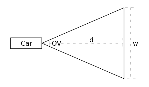
Figure 4 (crudely) illustrates a car with a forward-facing camera. The bottom row of pixels visible from the camera will be a narrow part of the road close to the vehicle. As you move up each for of pixels towards the row with the horizon, the physical area covered by that row of pixels will increase. The camera’s field of view (FOV), in degrees, has not changed, but the field of view in physical area has gone up. That means that the number of pixels per unit area decreases.

This decrease in resolution means that more distant objects have worse resolution than nearer objects. This isn’t exactly world-shaking news, but consider the task of lane location prediction for an autonomous vehicle. If the lane and lane markers get too small, then lane prediction will become impossible.

The area covered by the image at each row of pixels increases with distance, $d$. The physical width, $w$, is determined by:

$w = tan(FOV/2)*2d$

At 200m, a 120 FOV camera covers an area 693 meters wide. A 3.5m lane only fills about 0.5% of the image. A standard 1920 pixel wide camera image would use less than 10 pixels for that lane. That sounds okay–but what about the lane markers?

Lane markers are only about 10cm wide. That’s 0.015% of the image or a quarter of a pixel in the 1920 pixel wide example. A white lane marker on a black road will end up being about 1/4 of its expected brightness, which is probably okay under ideal conditions. However, when the marking is worn down or when there is glare on the asphalt from the sun or overhead lights on a wet surface the problem clearly becomes more difficult. In conclusion, you should expect performance to drop with distance almost linearly.

We’ve looked at two examples of how data can limit your DNN prediction quality. In ImageNet, bad or ambiguous labels will decrease performance. In autonomous vehicles, and other robotics applications, image quality can constrain your maximum performance. I recommend doing a quick estimate of your theoretical peak performance before starting any DNN work. Even if you find nothing terribly wrong with your data, you will at least know how high performance should be able to go, which is better than just guessing.