Learning and Regularization – Linear Functions

I was recently reading François Fleuret book, titled “The Little Book of Deep Learning.” It’s available online. I don’t have any complaints about it, so if you want a terse crash course on deep learning it’s a good choice. The brevity of the sections does mean that some nuance may escape a reader, and while I was reading an early section (1.2 to be exact) it occured to me that a deeper dive into some early concepts could benefit someone who is trying to understand deep neural networks (DNNs). This post will cover using small networks to approximate linear functions, but I hope some of the observations will give some useful insights into the ideas of regularization and overfitting.

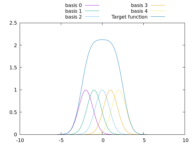
First, let’s review the problem from Fleuret’s book. Our task is to model a function that is a linear combination of other functions. More formally, $f(x) = \Sigma^K_{k=1}(w_{k}f_{k}(x))$, where $w_k$ is the weight of the $k^{th}$ basis function. Less formally, here is a picture:

To learn this function, we can have a neural network with five inputs, one for each basis function, and have it learn a weight for each input. This is a single layer neural network with five weights, and, since the basis functions are all linear, gradient descent will solve the problem perfectly. In fact, as long as the number of training samples is sufficient to solve the problem (five points for a conic, so we could change up the basis functions and still only require five), the DNN will solve this with arbitrary precision. End of story, we can’t overfit with the functions shown¹. Give it a shot.

But what if the basis functions aren’t provided? Now the neural network must learn a piecewise linear fit, using multiple straight lines from linear layers that take $x$ as an input to output an approximation of the desired curve. We will have to break out the multi-layer perceptron now.

With pytorch, we’ll get code like this:

def sample_curve(offset, spread, magnitude, x):
    """This will look like a normal distribution with maximum of the given magnitude."""
    return magnitude * 2**(-(x - offset)**2/spread)

# The basic example of overfitting from "The Little Book of Deep Learning" involves summing several curves into a larger curve
# The author discusses the example with Gaussian kernels, but let's talk about NNs

basis_functions = [functools.partial(sample_curve, -2 + offset, 1, 1) for offset in range(5)]

def correct_output(x):
    return sum([basis(x) for basis in basis_functions])

# Typical neural network with lots of parameters.
net = torch.nn.Sequential(
        torch.nn.Linear(1, 128),
        torch.nn.ReLU(),
        torch.nn.Linear(128, 128),
        torch.nn.ReLU(),
        torch.nn.Linear(128, 1))
optimizer = torch.optim.SGD(net.parameters(), lr=0.001, momentum=0.0)
loss_fn = torch.nn.MSELoss(reduction='sum')

net.train()

# First, let's just fit to 60 points from -2.5 to 1 and from 1 to 2.5.
xs = sorted([-2.5 + 1.5*random.random() for _ in range(30)] + [1 + 1.5*random.random() for _ in range(30)])
x_inputs = torch.tensor(xs).view((len(xs), 1))
sample_outputs = torch.tensor([[correct_output(x)] for x in xs])

for step in range(1000):
    optimizer.zero_grad()
    output = net.forward(x_inputs)
    loss = loss_fn(output, sample_outputs)
    loss.backward()
    optimizer.step()

net.eval()

# Get the final result across the full range
xs = [-2.5 + 0.05 * x for x in range(101)]
x_inputs = torch.tensor(xs).view((len(xs), 1))
output = net.forward(x_inputs)

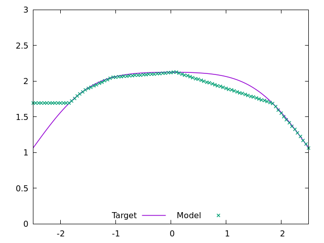
The result of training is in Figure 2.

Can we say that the model is overfit? Well…

Certainly the error is higher where it wasn’t trained, which was 40% of the data range. The fact that it’s a bit wrong there isn’t surprising, but I wouldn’t call this an “overfit” issue, because the existing data isn’t “pushing” the model to be worse in the unknown region. This is just an issue of lack of data².

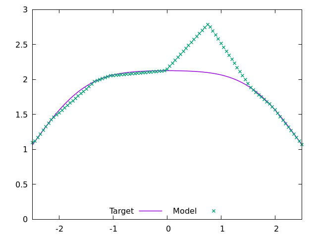
It would take very little data to solve this. Let’s just add a single training point in the range [-0.1,0.1].

# First, let's just fit to 60 points from -2.5 to 1, -0.1 to 0.1, and from 1 to 2.5.
xs = sorted([-2.5 + 1.5*random.random() for _ in range(30)] + [-0.1 + 0.2*random.random() for _ in range(1)] + [1 + 1.5*random.random() for _ in range(30)])

From Figure 3 we can see that just a tiny bit of data will fix our issue. If we truly had an “overfitting” issue, that would imply that the training data contradicts what was in the untrained area, but in fact the data ranges are copacetic.

So have we gotten everything we can from this example? Not yet, I think. Let’s spend a moment looking at how the model is learning to approximate this function – it will make it clear why I don’t think of these issues as “overfitting”.

Imagine, for a moment, that you were solving this problem with nothing but a linear network. At your disposal are a pair of linear layers with a ReLU in between. You are given a number of sample points from the function to model, and let’s say for simplicity’s sake that the number of sample points is the same as the number of weights in the linear layers. What do you do?

You build a piecewise linear fit, that’s what. Let’s consider the samples in order, from first to last along the x-dimension. We have to make an assumption about what we want the model output to be outside of the range of the sample points. For simplicity, let’s have the model output the y-value of the first sample when x is less than that sample’s location. It’s not perfect, but who can say what the function looks like outside of the sample range?

That decided, this is just a straight line. We can just set the weight and bias to 0 in the first layer and set the bias of the second linear layer to the sample’s y-value and be done.

# Our sorted samples with 9 elements
xs = sorted([-2.5 + 1.5*random.random() for _ in range(4)] + [-0.1 + 0.2*random.random() for _ in range(1)] + [1 + 1.5*random.random() for _ in range(4)])
sample_outputs = torch.tensor([[correct_output(x)] for x in xs])

# Our DNN with 16 weights in each linear layer.
net = torch.nn.Sequential(
        torch.nn.Linear(1, 8),
        torch.nn.ReLU(),
        torch.nn.Linear(8, 1))

with torch.no_grad():
    net[0].weight.fill_(0.)
    net[0].bias.fill_(0.)
    net[2].weight.fill_(0.)
    net[2].bias[0] = sample_outputs[0]

The rest of the points require actual effort. To go from the first sample to the second, we need the output of the network to have the slope $(sample\_outputs_1 - sample\_outputs_0)/(xs_1 - xs_0)$. Setting the weight of the first layer to the slope is almost right, but we have to deal with the slope hanging coming from the previous weight. Use the delta of the slopes instead of the slope itself.

One more thing. We don’t want to see that slope until after we have passed the first sample, so set the bias of the first layer to intercept $y=0$ at $x = xs_0$

That’s almost right, but if the slope is negative this won’t pass through the ReLU. To handle that case, set the weight to the negative of the slope in the first layer and then set the weight to -1 in the second layer.

Otherwise, the weight in the second layer should be 1. With some clever use of the abs and copysign functions to keep the code terse, those changes result in the following code:

    # Remember the slopes for delta slope calculations
    slopes = [0.]

    # Set all other weight and bias values to handle slopes for the rest of the points
    for i in range(1, len(xs)):
        slope = (sample_outputs[i]-sample_outputs[i-1]) / (xs[i]-xs[i-1])
        slopes.append(slope)
        delta_slope = slopes[-1] - slopes[-2]
        net[0].weight[i-1,0] = abs(delta_slope)
        net[0].bias[i-1] = -xs[i-1] * abs(delta_slope)
        net[2].weight[0,i-1] = math.copysign(1, delta_slope)

We end up with a decent fit, as seen in Figure 4. It’s wrong where we lacked data, but that is no fault of the approach.

Now, what would happen if we didn’t use all of the weight and bias values? Let’s add two more:

        # Add in two "bad" neurons to the linear layers
        target_slope = (sample_outputs[5] - sample_outputs[4]) - (xs[5] - xs[4])
        net[0].weight[8,0] = 1
        net[0].weight[9,0] = 2
        # The first one "turns on" after the first target point
        net[0].bias[8] = -xs[4]
        # The second one "turns on" halfway to the second
        net[0].bias[9] = 2 * -(xs[4] + (xs[5]-xs[4])/2.0)
        net[2].weight[0,8] = 1
        net[2].weight[0,9] = -1
        # The outputs of the two neurons cancel when x = target_xs[1]
        # To prevent adding error into the network output we need to add a positive slope to the network at target_xs[1]
        new_slope = slopes[6] + 1
        new_delta = new_slope - slopes[5]
        net[0].weight[5,0] = abs(new_delta)
        net[0].bias[5] = -xs[5] * abs(new_delta)
        net[2].weight[0,5] = math.copysign(1, new_delta)

Will gradient descent fix this?

    loss_fn = torch.nn.MSELoss(reduction='sum')
    with torch.no_grad():
        output = net.forward(torch.tensor(xs).view((len(xs), 1)))
        loss = loss_fn(output, sample_outputs)
        print(f"Loss is {loss}")

The answer is no³. The real solution is regularization. The mechanics of how a regularizing function can fix this are complicated, depending upon the function. For the simplest case, consider assigning a penalty to all weights (the “weight_decay” option in torch.optim.SGD). Those weights do not cause any loss, but changing them will not increase loss either. A weight decay will slowly drive them to 0, with the weight of the fifth neuron changing back to its value before we added them into the network.

So let’s summarize. Linear functions don’t suffer from what I think of as overfitting. If your training data is sparse though, it is possible for the random initialization of a network to give you bad (perhaps even spiky) outputs in those unexplored areas. This is all luck: depending upon the initial randomized parameters of the model and the distributions of your training data you may never see a problem. If you do though, this is where regularization can come to the rescue. I’ll leave the mechanics of that to a different post, but it’s safe to say that every modern training regime includes regularization.