<!-- Abstract: You may have heard that overfitting is a problem in machine learning. You may have even heard that regularization fixes the problem. But what is regularization? Regularization techniques pre-date modern machine learning, including deep neural networks. Although deep neural networks are surprisingly robust to overfitting, regularization is still an essential part of neural network training. In this talk, we will look at overfitting and regularization in neural networks. How do they resist overfitting? What techniques can we use to regularize neural networks? What are some of the problems that regularization solves? --> # Regularization ## in Deep Neural Networks Bernhard Firner 2025-03-10 --- ## Neural Networks in the 90s 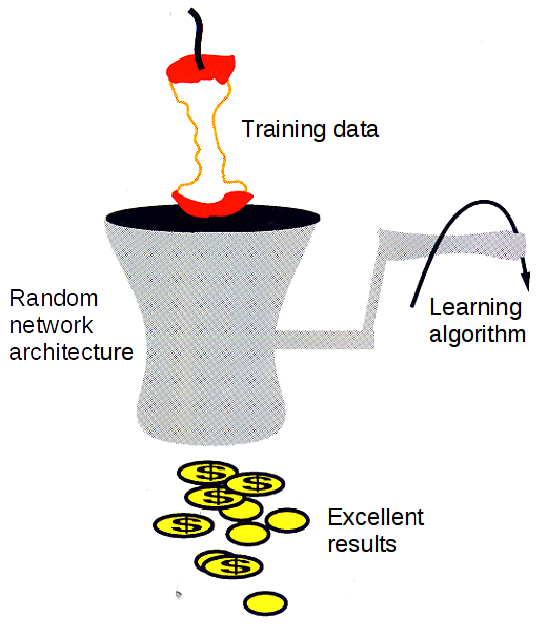 Note: I got this from Larry Jackel, who gathered an enormously talented group at Bel Labs; people such as Yoshua Bengio, Yann LeCun, Vladimir Vapnik, and many others. Larry complained that people would expect magic from learning systems, without considering details about the data or what algorithms they used, and would be surprised when they didn't print money. --- ## Neural Networks Today <img src="./figures/NeuralNetworkMagicByBenFirner.png" style="height: 750px" /> Note: Today the biggest difference is that AI can draw the diagram. With open source frameworks, github repositories, and freely available datasets, you can quickly apply the latest and greatest research to your own problem, and quickly get terrible results. It's like giving an unskilled baker into the kitchen with all the right ingredients: theoretically you have sufficient items for success, but in reality you'll get something inedible. I'm not saying anything bad about someone who can't bake, or an undergraduate who doesn't understand why the from a github repo doesn't work -- both baking and machine learning are hard. --- ## Well-Recognized Problem > By itself, this enhanced training recipe increased the performance of the ResNet-50 model from 76.1% to 78.8% (+2.7%), implying that a significant portion of the performance difference between traditional ConvNets and vision Transformers may be due to the training techniques. [A ConvNet for the 2020s](https://arxiv.org/abs/2201.03545) Note: Don't just take my word for it -- active researchers have realized the same thing. When something new hits the scenes, people scramble to produce improved results with it. Taking the time to pinpoint what exactly made the results better is laborious and sometimes unrewarding. In some cases, the thing grabbing everyone's attention is not actually the source of the improved results. --- ## Goal for Today * Convince you that neural networks are wonderful, but flawed tools * Teach you a couple of flaws so that you can deal with them --- ## What is a Regularizer? * Regularizers are tools or techniques to "simplify" statistical models * Reduce "overfitting" to noise in training * Improve generalization * They've long been a part of statistical methods --- ## What is Overfitting? * Failure to generalize due to mismatch between data and model complexity \ <sub style="font-size: 0.6em">By Chabacano - Own work, CC BY-SA 4.0, https://commons.wikimedia.org/w/index.php?curid=3610704</sub> --- ## Regularization in Neural Networks * Reuses some techniques from other statistical methods * Neural networks are used in new tasks, so new regularization techniques were invented We'll begin with a traditional example. --- ## Some Prerequisites * Going to assume that you know something about statistical modelling * e.g. you know about "curve fitting" * Ideally, you know the components of an artificial neural network * Examples will be in Python * Neural networking in PyTorch, but experience isn't required Note: Before diving into some code, let me verify that we can speak the same language. I'll go through some code examples if necessary. --- ## Least Squares Overfitting ```python [|2-5,8,9|8,13|14|16-22] import numpy def sample_curve(x): """Produce a curve for fitting examples.""" return 2**(-10*(x - 0.5)**2) # The x and y points along a curve x_samples = [0.05 * x for x in range(21)] y_samples = [sample_curve(x) for x in x_samples] # The perfect solution to a noiseless set of points. # We will solve with a as many coefficients as samples A = numpy.vander(x_samples, N=20, increasing=True) coef = numpy.linalg.lstsq(A, y_samples, rcond=-1)[0] # Print out the samples and our fit line print("x, y samples, fit") # Also plot some extra points to see how the fit generalizes between the training points x_samples = [0.025 * x for x in range(41)] y_samples = [sample_curve(x) for x in x_samples] for idx, point in enumerate(zip(x_samples, y_samples)): prediction = sum([c * point[0]**i for i, c in enumerate(coef)]) print(f"{point[0]}, {point[1]}, {prediction}") ``` Note: Don't worry about the code too much, it's here so you can play with the example. --- ## Without Noise  --- ## Adding Noise ```python [|10-11|14-17|18-29] import numpy def sample_curve(x): """Produce a curve for fitting examples.""" return 2**(-10*(x - 0.5)**2) # The x and y points along a curve x_samples = [0.05 * x for x in range(21)] y_samples = [sample_curve(x) for x in x_samples] noise_generator = numpy.random.default_rng() noise = numpy.random.standard_normal(len(y_samples)) * 0.05 # The perfect solution to a noiseless set of points. A = numpy.vander(x_samples, N=5, increasing=True) coef = numpy.linalg.lstsq(A, y_samples + noise, rcond=-1)[0] A_over = numpy.vander(x_samples, N=20, increasing=True) coef_over = numpy.linalg.lstsq(A_over, y_samples + noise, rcond=-1)[0] # Print out the samples and our fit line print("x, y samples, y noise, fit, overfit") # Also plot some extra points to see how the fit generalizes between the training points x_samples = [0.025 * x for x in range(41)] y_samples = [sample_curve(0.5, 0.1, 1, x) for x in x_samples] for idx, point in enumerate(zip(x_samples, y_samples)): prediction = sum([c * point[0]**i for i, c in enumerate(coef)]) overfit_prediction = sum([c * point[0]**i for i, c in enumerate(coef_over)]) if idx % 2 == 0: print(f"{point[0]}, {point[1]}, {point[1] + noise[idx//2]}, {prediction}, {overfit_prediction}") else: print(f"{point[0]}, {point[1]}, none, {prediction}, {overfit_prediction}") ``` --- ## Least Squares with Noise  The "overfit" line touches each point, but sacrifices simplicity.\ The "fit" line has a quarter as many parameters but is a better approximation. --- ## Regularizers in Neural Networks * Parameters vastly outnumber the problem dimension * Do we see the same overfitting problem? * Not quite. -v- ## A Quick Primer on Linear NNs * The basic building block of a neural network is an artificial neuron * Has a `weight`, $w$, for each of $k$ inputs * Also has a `bias`, $b$ * Given input, $x_1$ ... $x_k$, the output is $b + \sum^k_{i=1}w_{i}x_i$ * A `linear layer` with $n$ outputs has $n$ neurons. * Each neuron in the layer uses the same inputs * Also called a `fully connected` layer ```torch torch.nn.Linear(1, 1000), ``` -v- ## Connecting Layers * Linear layers can be directly connected * Experience shows this is not optimal * All outputs would be linear responses to the input * Putting a `nonlinearity` between layers allows more complex functions ```python net = torch.nn.Sequential( torch.nn.Linear(1, 1000), torch.nn.ReLU(), torch.nn.Linear(1000, 1000), torch.nn.ReLU(), torch.nn.Linear(1000, 1)) ``` -v- ## ReLU  Rectified Linear Unit function $f(x) = max(0, x)$ -v- ## Toy Example * Let's say we want to output this function: <img src="./figures/toy_example2.png" style="height: 425px" /> -v- ## Toy Example Code ```python import torch net = torch.nn.Sequential( # 1 inputs, 2 output torch.nn.Linear(1, 2), torch.nn.ReLU(), # 2 inputs, 1 outputs torch.nn.Linear(2, 1)) # We are directly changing the model parameters, so we need to tell PyTorch # that we don't treat this as learning with torch.no_grad(): # There are two bias values in the first layer, since there are two outputs net[0].bias[0] = 1 net[0].bias[1] = -1 # There are two weights in the first layer, for the two outputs # The first index of a linear layer's weights is the output number, # the second is the input number. net[0].weight[0,0] = 1 net[0].weight[1,0] = 2 # The first two layers of the network have two outputs: # f_1(x) = ReLU(1 + x) # f_2(x) = ReLU(-1 + 2x) # There is one bias value in the third layer, for the one output. net[2].bias[0] = 0.25 # There are two weight values in the first layer, one for each input. net[2].weight[0,0] = 0.75 net[2].weight[0,1] = -0.75 # The network performs g(x) = 0.25 + 0.75f_1(x) - 0.75f_2(x) # g(x) = 0.25 + 0.75*RelU(1 + x) - 0.75*ReLU(-1 + 2x) for x in [-1 + inc*0.25 for inc in range(9)]: print(f"g({x}) = {net.forward(torch.tensor([x]))}") ``` -v- ## Learning with Gradient Descent * You typically train a neural network with pairs of inputs and outputs * The error, or `loss`, is the difference between the network output and the desired output * The loss function could be mean squared error, absolute error, or others ```python loss_fn = torch.nn.MSELoss(reduction='sum') ``` -v- ## Loss ```python output = net.forward(x_inputs) loss = loss_fn(output, y_targets) loss.backward() ``` * The output calculation is called the `forward` pass * In the `backward` pass, you assign a responsibility for the error to each weight and bias * This is called the `gradient` * Calculated via the derivative * [Wikipedia link on backpropagation](https://en.wikipedia.org/wiki/Backpropagation) -v- ## Parameter Updates * Once a gradient (blame) is assigned to all weight and bias values, they are updated * Could be simple * multiplying all gradients by a constant and add to the parameters * The constant is called the `learning rate` ```python optimizer.zero_grad() output = net.forward(x_inputs) loss = loss_fn(output, y_targets) loss.backward() optimizer.step() ``` -v- ## Surprisingly Robust <!-- TODO FIXME: Transition slide back to the main topic --> --- ## Really? Let's take an example ```python [|4-13|20-25|27-28|32-41|49-59] import numpy import torch def sample_curve(x): """Produce a curve for fitting examples.""" return 2**(-10*(x - 0.5)**2) # The x and y points along a curve x_samples = [0.05 * x for x in range(21)] y_samples = [sample_curve(x) for x in x_samples] noise_generator = numpy.random.default_rng() noise = numpy.random.standard_normal(len(y_samples)) * 0.05 ################ # For better repeatability torch.random.manual_seed(0) net = torch.nn.Sequential( torch.nn.Linear(1, 1000), torch.nn.ReLU(), torch.nn.Linear(1000, 1000), torch.nn.ReLU(), torch.nn.Linear(1000, 1)) # Results are less predictable without momentum optimizer = torch.optim.SGD(net.parameters(), lr=0.004, momentum=0.05) loss_fn = torch.nn.MSELoss(reduction='sum') net.train() x_inputs = torch.tensor(x_samples).view((len(x_samples), 1)) y_targets = torch.tensor(y_samples).view((len(y_samples), 1)) # Train for 4000 steps for step in range(4000): optimizer.zero_grad() output = net.forward(x_inputs) loss = loss_fn(output, y_targets) loss.backward() optimizer.step() # Note: We could stop early if we achieve good enough results # There is no harm is training for longer # if loss < 0.005: # break net.eval() # Print out the samples and our predictions print("x, y samples, y noise, prediction") # Also plot some extra points to see how the fit generalizes between the training points x_samples = [0.025 * x for x in range(41)] y_samples = [sample_curve(x) for x in x_samples] prediction = net(torch.tensor(x_samples).view((len(x_samples), 1))).flatten().tolist() for idx, point in enumerate(zip(x_samples, y_samples)): if idx % 2 == 0: print(f"{point[0]}, {point[1]}, {point[1] + noise[idx//2]}, {prediction[idx]}") else: print(f"{point[0]}, {point[1]}, none, {prediction[idx]}") ``` --- ## NN with Noisy Data 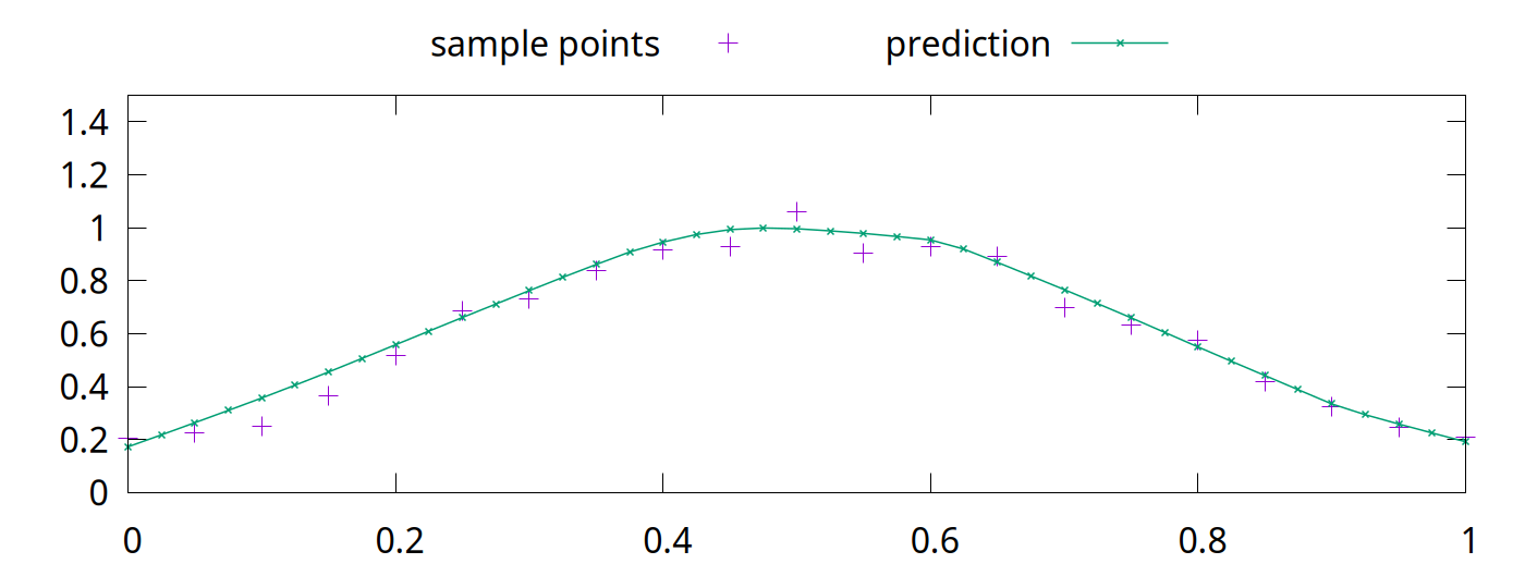 Magic! --- ## Why Does This Work? * Short answer: *Gradient Descent* is *magic* * Longer answer is that success will vary: * with the kind of noise * with the task * Here, the local minima resists moving into a tortured function * Local minima is where the NN parameters get "stuck" * Non-optimal solution, but often simpler * The output is a piecewise fit of 1000 neurons, which is naturally smooth <!-- Make a drop down slide to illustrate that mechanic --> * Despite this success, regularizers are *vital* for deep learning --- ## Deep Neural Networks ### (DNNs) * Practitioners *do not* try to use smaller models * Instead, we (generally) use the largest model feasible * Why? * Unexpectedly, larger models generalize better than smaller models * Don't think this means that DNNs are *immune* to overfitting issues \ \ \ Further reading: [The Loss Surfaces of Multilayer Networks](https://arxiv.org/abs/1412.0233) <!-- Make a drop down with some images from Anna's paper --> --- ## Common Regularization Techniques * L2 penalty * Penalizes the network for having high-magnitude parameters * Dropout * Portions of network layers are randomly ignored during training * Stochastic Depth * Entire layers of the network are randomly ignored during training * Label Smoothing * Data augmentation * Changes to the learning target --- ## L2 Penalty: Motivations L2 penalties simplify the model outside of our training range 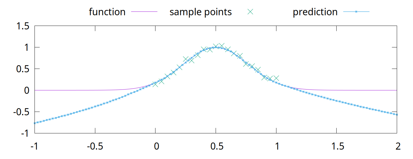 The previous model was trained without an L2 penalty\ Outside of the training domain, it diverges far from the nearest points. --- ## The L2 Penalty * Add the square of each weight in the network to the loss * Formally: * $\sum^k_{i=1} w_{i}^2$ * The loss is the derivative of that: * $2\sum^k_{i=1} w_{i}$ * Multiplied by a factor, $\alpha$ --- ## Adding L2 to Our Loss * Conceptually, just add the sum of the parameters to the loss * Note, PyTorch's optimizer does other things with the loss value * Momentum operates on the loss value, for example. * Pass $\alpha$ to the `weight_decay` option in PyTorch's SGD optimizer * We'll arbitrarily choose $\alpha = 0.08$ * If we set the value extremely high it will force all weights to 0 * Results in a flat line ```python optimizer = torch.optim.SGD(net.parameters(), lr=0.004, momentum=0.05, weight_decay=0.08) ``` --- ## L2 Penalty Results With L2, results are improved outside of the training domain. 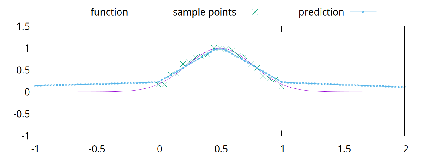 The L2 penalty has more utility than this. <!-- TODO FIXME Add in a histogram of the weights with and without L2 --> --- ## L2 Continued 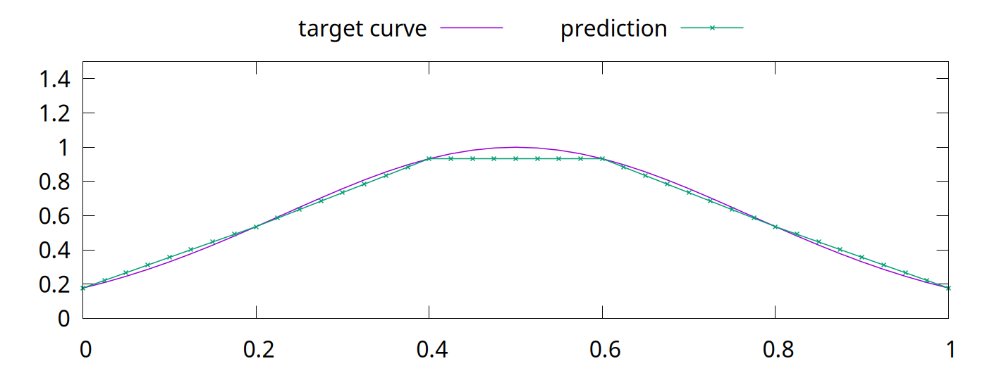 This is a piecewise fit using a tiny neural network. ```python net = torch.nn.Sequential( torch.nn.Linear(1, 6), torch.nn.ReLU(), torch.nn.Linear(6, 1)) ``` <!-- Also talk about pruning, maybe in a digression --> -v- ## Building a Solution Let's build a solution so we can break it ```python [|4-10|17-20|25-31|34-37|39|39-41|41-43|44-45|46-47|49|55-69|74-81] import math import torch def sample_curve(x): """Produce a curve for fitting examples.""" return 2**(-10*(x - 0.5)**2) # The x and y points along a curve x_samples = [0.2 * x for x in range(6)] y_samples = [sample_curve(x) for x in x_samples] ################ # For better repeatability torch.random.manual_seed(0) net = torch.nn.Sequential( torch.nn.Linear(1, 6), torch.nn.ReLU(), torch.nn.Linear(6, 1)) # Instead of training the model, we will set the parameters so that the output # intercepts each of the training points. # This turns off gradient calculations since we aren't do learning. with torch.no_grad(): # Initialize all parameters to 0. net[0].bias.fill_(0.) net[0].weight.fill_(0.) net[2].bias.fill_(0.) net[2].weight.fill_(0.) # Remember the slopes for delta slope calculations slopes = [0.] # Set all other weight and bias values to handle slopes for the rest of the points for i in range(1, len(x_samples)): # Calculate the changes in slope required to go from one point to the next slope = (y_samples[i]-y_samples[i-1]) / (x_samples[i]-x_samples[i-1]) slopes.append(slope) delta_slope = slopes[-1] - slopes[-2] # The weight for the next parameter will be the delta slope net[0].weight[i-1,0] = abs(delta_slope) # Set the bias value so that the output will be <0 before this training point net[0].bias[i-1] = -x_samples[i-1] * abs(delta_slope) # In the second linear layer, set the correct sign for the slope net[2].weight[0,i-1] = math.copysign(1, delta_slope) # Set the bias value to match the first y value of the training points net[2].bias[0] = y_samples[0] ################ # See what gradient descent can do net.train() loss_fn = torch.nn.MSELoss(reduction='sum') x_inputs = torch.tensor(x_samples).view((len(x_samples), 1)) y_targets = torch.tensor(y_samples).view((len(y_samples), 1)) output = net.forward(x_inputs) loss = loss_fn(output, y_targets) print(f"Initial loss is {loss}") optimizer = torch.optim.SGD(net.parameters(), lr=0.004, momentum=0.05) # Train for 4000 steps for step in range(4000): #printCurrentModel(step=step, xs=xs, x_inputs=x_inputs, net=net) optimizer.zero_grad() output = net.forward(x_inputs) loss = loss_fn(output, y_targets) loss.backward() optimizer.step() print(f"Final loss is {loss}") ################ net.eval() # Print out the samples and our predictions print("x, y samples, prediction") # Also plot some extra points to see how the fit generalizes between the training points x_samples = [0.025 * x for x in range(41)] y_samples = [sample_curve(x) for x in x_samples] prediction = net(torch.tensor(x_samples).view((len(x_samples), 1))).flatten().tolist() for idx, point in enumerate(zip(x_samples, y_samples)): print(f"{point[0]}, {point[1]}, {prediction[idx]}") ``` Loss is 1.1013412404281553e-13 --- ## Now With an Error 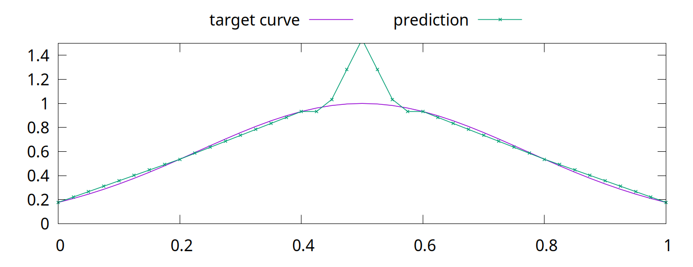 Added 3 more neurons to create the bump. ```python net = torch.nn.Sequential( torch.nn.Linear(1, 9), torch.nn.ReLU(), torch.nn.Linear(9, 1)) ``` -v- ## Adding an Error We can make the network worse without changing the loss: ```python [|18-21|52-56|57-60|61-64|65-68] import math import torch def sample_curve(x): """Produce a curve for fitting examples.""" return 2**(-10*(x - 0.5)**2) # The x and y points along a curve x_samples = [0.2 * x for x in range(6)] y_samples = [sample_curve(x) for x in x_samples] ################ # For better repeatability torch.random.manual_seed(0) # Larger model so we can insert errors net = torch.nn.Sequential( torch.nn.Linear(1, 9), torch.nn.ReLU(), torch.nn.Linear(9, 1)) # Instead of training the model, we will set the parameters so that the output # intercepts each of the training points. # This turns off gradient calculations since we aren't do learning. with torch.no_grad(): # Initialize all parameters to 0. net[0].bias.fill_(0.) net[0].weight.fill_(0.) net[2].bias.fill_(0.) net[2].weight.fill_(0.) # Remember the slopes for delta slope calculations slopes = [0.] # Set all other weight and bias values to handle slopes for the rest of the points for i in range(1, len(x_samples)): # Calculate the changes in slope required to go from one point to the next slope = (y_samples[i]-y_samples[i-1]) / (x_samples[i]-x_samples[i-1]) slopes.append(slope) delta_slope = slopes[-1] - slopes[-2] # The weight for the next parameter will be the delta slope net[0].weight[i-1,0] = abs(delta_slope) # Set the bias value so that the output will be <0 before this training point net[0].bias[i-1] = -x_samples[i-1] * abs(delta_slope) # In the second linear layer, set the correct sign for the slope net[2].weight[0,i-1] = math.copysign(1, delta_slope) # Set the bias value to match the first y value of the training points net[2].bias[0] = y_samples[0] # Now add in an egregious error in the middle of the points error_begin = x_samples[2] + (x_samples[3] - x_samples[2])/5 error_end = x_samples[3] - (x_samples[3] - x_samples[2])/5 error_middle = (error_begin + error_end) / 2 error_slope = 10 # Go egregiously wrong between error_begin and error_middle net[0].weight[-3] = error_slope net[0].bias[-3] = -error_begin * error_slope net[2].weight[0,-3] = 1 # Now cancel the error slope by going back down at twice the rate net[0].weight[-2] = 2 * error_slope net[0].bias[-2] = -error_middle * 2 * error_slope net[2].weight[0,-2] = -1 # Now cancel out what we've done so the slope is the same as before net[0].weight[-1] = error_slope net[0].bias[-1] = -error_end * error_slope net[2].weight[0,-1] = 1 # See what gradient descent can do net.train() loss_fn = torch.nn.MSELoss(reduction='sum') x_inputs = torch.tensor(x_samples).view((len(x_samples), 1)) y_targets = torch.tensor(y_samples).view((len(y_samples), 1)) output = net.forward(x_inputs) loss = loss_fn(output, y_targets) print(f"Initial loss is {loss}") optimizer = torch.optim.SGD(net.parameters(), lr=0.004, momentum=0.05) # Train for 4000 steps for step in range(4000): optimizer.zero_grad() output = net.forward(x_inputs) loss = loss_fn(output, y_targets) loss.backward() # If you want to inspect the gradients: #if step == 0: # print(f"Grads are {[p.grad for p in net.parameters()]}") optimizer.step() print(f"Final loss is {loss}") ################ net.eval() # Print out the samples and our predictions print("x, y samples, prediction") # Also plot some extra points to see how the fit generalizes between the training points x_samples = [0.025 * x for x in range(41)] y_samples = [sample_curve(x) for x in x_samples] prediction = net(torch.tensor(x_samples).view((len(x_samples), 1))).flatten().tolist() for idx, point in enumerate(zip(x_samples, y_samples)): print(f"{point[0]}, {point[1]}, {prediction[idx]}") ``` --- ## Will Gradient Descent Fix It? No. The loss is fantastic. Initial loss is 2.8066438062523957e-13 After running training on the network with the bump:\ Final loss is 3.597122599785507e-14 --- ## Now Add L2 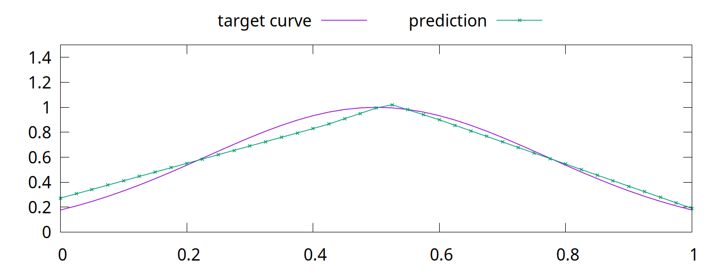 It isn't perfect, but it improves areas with sparse training data. What about biased or incomplete data? --- ## Data Bias Great example from [Google research](https://research.google/blog/inceptionism-going-deeper-into-neural-networks/) into neural network visualization in 2015: > [T]his reveals that the neural net isn’t quite looking for the thing we thought it was. For example, here’s what one neural net we designed thought dumbbells looked like: <img src="./figures/dumbbells.png" style="height: 300px" /> Arms are correlated with dumbbells, hence the confusion. --- ## Correlations * DNNs mine for signals that are correlated with a desired output * e.g. eyes and noses are correlated with faces * Some correlations are weak, some are strong, and some are just spurious * A hard problem; living creatures can be fooled by data bias as well <img src="./figures/Automeris_ioPCCA20040704-2975AB1.jpg" style="height: 600px" /> <img src="./figures/Glaucidium_californicum_Verdi_Sierra_Pines_2_(detail).jpg" style="height: 600px" /> <sub style="font-size: 0.5em">By Patrick Coin (Patrick Coin) - Photograph taken by Patrick Coin, CC BY-SA 2.5, https://commons.wikimedia.org/w/index.php?curid=768361<br/> By Tim from Ithaca - Northern Pygmy Owl, CC BY 2.0, https://commons.wikimedia.org/w/index.php?curid=96044504</sub> --- ## Dropout * Different benefits have been ascribed to [Dropout](https://arxiv.org/abs/1207.0580) * From early papers, prevents "co-adaptation" of features * Creates a superposition of smaller DNNs within a larger DNN * Comes with the same advantages as an ensemble * This is a more recent explanation * Dropout makes models prefer stronger signals over weaker signals * This is a "makes it happen faster" effect * Dropout unbiases preferences for similar signals --- ## What is Dropout? * During training, randomly ignore some neurons * For example, given neurons a, b, c, and d, drop half at each training step: 1. $f(x) = a + d$ <!--.element: class="fragment" data-fragment-index="1" --> 1. $f(x) = a + c$ <!--.element: class="fragment" data-fragment-index="2" --> 1. $f(x) = b + c$ <!--.element: class="fragment" data-fragment-index="3" --> 1. $f(x) = a + c$ <!--.element: class="fragment" data-fragment-index="4" --> * When training is done, use them all <!--.element: class="fragment" data-fragment-index="5" --> * Now there are four numbers instead of two, so divide by half to preserve average outputs magnitude <!--.element: class="fragment" data-fragment-index="5" --> $f(x) = (a + b + c + d)/2$ <!--.element: class="fragment" data-fragment-index="5" --> --- ## Realistic Inputs Suppose that your training data has two signals that are always the same. ```python [|7-13|15-28|30-31|35-42|46-52] import random import torch # For better repeatability torch.random.manual_seed(0) # Imagine that the inputs represent features in an image net = torch.nn.Sequential( torch.nn.Linear(2, 100), torch.nn.ReLU(), torch.nn.Linear(100, 100), torch.nn.ReLU(), torch.nn.Linear(100, 1)) # Our training set. def make_input_outputs(size): with torch.no_grad(): # Make a batch of inputs that is just the same pairs of numbers inputs = torch.empty([size, 1]).uniform_(0, 1).repeat(1, 2) outputs = inputs[:,0].view((size, 1)) for idx in range(size): # 1/1000 chance that a signal is missing. if random.random() < 0.001: inputs[idx,0] = 0 if random.random() < 0.001: inputs[idx,1] = 0 return inputs, outputs optimizer = torch.optim.SGD(net.parameters(), lr=0.004, momentum=0.05, weight_decay=0.01) loss_fn = torch.nn.MSELoss(reduction='sum') net.train() # Train for a long time. for step in range(10000): x_inputs, y_targets = make_input_outputs(64) optimizer.zero_grad() output = net.forward(x_inputs) loss = loss_fn(output, y_targets) loss.backward() optimizer.step() net.eval() # Probe the network to test how it learned. print("input a, input b, output") for a in range(101): for b in range(101): probe = torch.tensor([a/100, b/100]) output = net.forward(probe) print(f"{a/100}, {b/100}, {output.item()}") ``` --- ## Biased Outputs 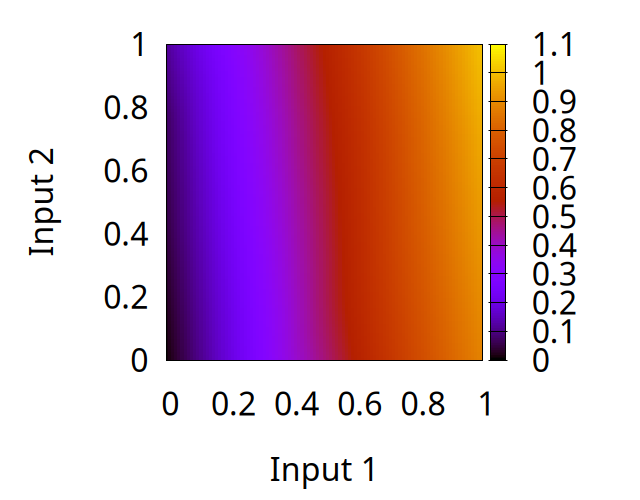 Seems to care more about input 1 than input 2. Why? Inputs 1 and 2 were copies, so why does the network treat them differently? --- ## With Dropout ```python [|11,14] import random import torch # For better repeatability torch.random.manual_seed(0) # Imagine that the inputs represent features in an image net = torch.nn.Sequential( torch.nn.Linear(2, 100), torch.nn.ReLU(), torch.nn.Dropout(0.5), torch.nn.Linear(100, 100), torch.nn.ReLU(), torch.nn.Dropout(0.5), torch.nn.Linear(100, 1)) # Our training set. def make_input_outputs(size): with torch.no_grad(): # Make a batch of inputs that is just the same pairs of numbers inputs = torch.empty([size, 1]).uniform_(0, 1).repeat(1, 2) outputs = inputs[:,0].view((size, 1)) for idx in range(size): # 1/1000 chance that a signal is missing. if random.random() < 0.001: inputs[idx,0] = 0 if random.random() < 0.001: inputs[idx,1] = 0 return inputs, outputs optimizer = torch.optim.SGD(net.parameters(), lr=0.004, momentum=0.05, weight_decay=0.01) loss_fn = torch.nn.MSELoss(reduction='sum') net.train() # Train for a long time. for step in range(10000): x_inputs, y_targets = make_input_outputs(64) optimizer.zero_grad() output = net.forward(x_inputs) loss = loss_fn(output, y_targets) loss.backward() optimizer.step() net.eval() # Probe the network to test how it learned. print("input a, input b, output") for a in range(101): for b in range(101): probe = torch.tensor([a/100, b/100]) output = net.forward(probe) print(f"{a/100}, {b/100}, {output.item()}") ``` --- ## Unbiased Outputs 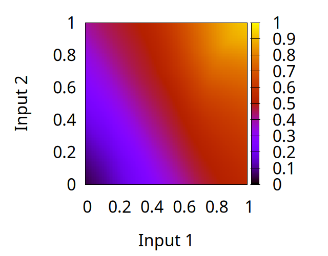 --- ## Other Approaches * Stochastic Depth * Label Smoothing * More data * Change the target or loss function --- ## Wrapup * Neural networks do have flaws * But incredibly powerful * You need to learn how they fail because the real world is difficult <!-- [A ConvNet for the 2020s](https://arxiv.org/abs/2201.03545) [More ConvNets in the 2020s: Scaling up Kernels Beyond 51x51 using Sparsity](https://arxiv.org/abs/2207.03620) [ConvNeXt V2: Co-designing and Scaling ConvNets with Masked Autoencoders](https://arxiv.org/abs/2301.00808) -->